\[
\require{physics}
\]
理想破壊強度
完全に欠陥のない結晶を、原子間結合そのものを引きちぎるには、どれくらいの応力が必要か? という話。
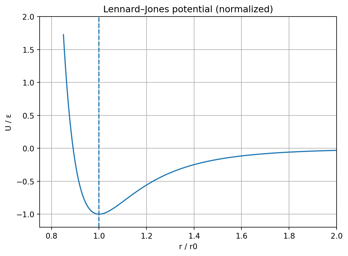
とりあえずなモデルとして、 Lennard–Jones ポテンシャルを考える。
 出典: https://en.wikipedia.org/wiki/Lennard-Jones_potential
ここで考えるべきは、極小点より右側だけ。破壊しようと思うのなら、それぞれの距離に対応した力を考えないといけない。
\[
F(r) = -\frac{dU}{dr}
\]
この原子間力を凝縮力と呼んでいて、単位面積あたりにして考えると応力になる。
具体的には次のような形になる。まず、Lennard–Jones ポテンシャルは、
\[
U(r) = 4\epsilon \left[ \left( \frac{\sigma}{r} \right)^{12} - \left( \frac{\sigma}{r} \right)^6 \right]
\]
という形で書かれる。ここで、\(\epsilon\) は井戸の深さ、\(\sigma\) は長さスケール。応力とかではないので注意!
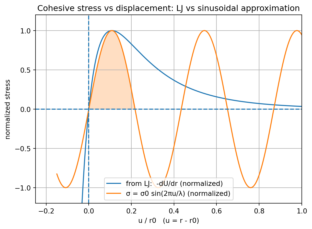
で、これを微分して力に変換すると、
\[
F(r) = -\frac{dU}{dr} = 24\epsilon \left[ \frac{2\sigma^{12}}{r^{13}} - \frac{\sigma^6}{r^7} \right]
\]
となる。わけで、実際にこれをグラフに起こしたら次のようになる。
コードはこちら
import numpy as np
import matplotlib.pyplot as plt

# --- Parameters (dimensionless) ---
eps = 1.0          # LJ井戸の深さ
sigma_LJ = 1.0     # LJの長さスケール
r0 = 2**(1/6) * sigma_LJ  # 平衡距離 (LJの最小点)

# 距離 r の範囲
r = np.linspace(0.85*r0, 2.8*r0, 1200)

# Lennard–Jones potential U(r)
U = 4*eps*((sigma_LJ/r)**12 - (sigma_LJ/r)**6)

# Cohesive force: F = -dU/dr
dUdr = np.gradient(U, r)
F = dUdr

# 応力っぽくする(形の比較用に最大引張を1に正規化)
F_tensile = np.clip(F, 0, None)
Fmax = F_tensile.max()
sigma_from_LJ = F / Fmax   # “stress-like” (dimensionless)

# 変位 u = r - r0
u = r - r0

# sin近似:ピーク位置をLJの引張ピークに合わせて λ を決める
peak_idx = np.argmax(F_tensile)
u_peak = u[peak_idx]
lam = 4*u_peak if u_peak > 0 else r0   # sinの最大が u=λ/4 なので λ=4u_peak
sigma0 = 1.0
sigma_sin = sigma0 * np.sin(2*np.pi*u/lam)

# --- Plot 1: LJ potential ---
plt.figure()
plt.plot(r/r0, U/eps)
plt.axvline(1.0, linestyle='--')
plt.xlabel("r / r0")
plt.ylabel("U / ε")
plt.title("Lennard–Jones potential (normalized)")
plt.xlim(0.75, 2.0)
plt.ylim(-1.2, 2.0)
plt.grid(True)

# --- Plot 2: cohesive stress vs displacement ---
plt.figure()
plt.plot(u/r0, sigma_from_LJ, label="from LJ:  -dU/dr (normalized)")
plt.plot(u/r0, sigma_sin, label="σ = σ0 sin(2πu/λ) (normalized)")
u_norm = u / r0
start_idx = np.argmax(u >= 0)
cross_rel = np.where((u[start_idx + 1:] > 0) & (sigma_sin[start_idx + 1:] <= 0))[0]
if cross_rel.size:
    end_idx = start_idx + 1 + cross_rel[0]
    fill_mask = (u_norm >= u_norm[start_idx]) & (u_norm <= u_norm[end_idx])
    plt.fill_between(
        u_norm,
        sigma_sin,
        0,
        where=fill_mask,
        color="C1",
        alpha=0.25,
        interpolate=True,
    )
plt.axhline(0.0, linestyle='--')
plt.axvline(0.0, linestyle='--')
plt.xlabel("u / r0   (u = r - r0)")
plt.ylabel("normalized stress")
plt.title("Cohesive stress vs displacement: LJ vs sinusoidal approximation")
plt.xlim(-0.25, 1)
plt.ylim(-1.2, 1.2)
plt.grid(True)
plt.legend()

plt.show()
ところが、 \(F\) はめっちゃ面倒なので、近似した形として
\[
\sigma(u) = \sigma_0 \sin\left( \frac{2\pi u}{\lambda} \right)
\]
を使うことになる。この時点から力から応力に変換して考えている。ここで、\(\sigma_0\) は最大応力、\(\lambda\) は原子間距離スケールに対応する長さ、\(u\) は変位を表す。
それで、 \(\lambda\) は長さの単位を持つけど、とりあえずあってそうな値を入れてるだけのフィッティング係数である。
弾性領域、つまりこのサインカーブの最初の方では、
\[
\begin{aligned}
\sigma(u) &= E \frac{u}{r_0} = \sigma_0 \frac{2\pi}{\lambda} u \\
\sigma_0 &= \frac{E \lambda}{2\pi r_0}
\end{aligned}
\]
また、このグラフのオレンジで囲われた部分が、破壊に必要なエネルギーに対応するので、表面エネルギーの2倍 \(2\gamma\) に等しい。すなわち、
\[
\begin{aligned}
2\gamma &= \int_0^{\lambda/2} \sigma(u) du \\
&= \sigma_0 \int_0^{\lambda/2} \sin\left( \frac{2\pi u}{\lambda} \right) du \\
&= \sigma_0 \cdot \frac{\lambda}{\pi}
\end{aligned}
\]
これらを組み合わせると、
\[
\sigma_0 = \sqrt{\frac{E \gamma}{r_0}} \sim \frac{E}{10}
\]
という式が得られる。これが理想破壊強度の見積もり式であるが、オーダーに関しては実際の値に比べて \(1/100\) 〜 \(1/1000\) 程度になることが知られている。
この理由としては、
- 塑性変形の介入。つまり、延性破壊が起きる。
- 化学的効果。不純物や環境要因によるもの。
- 欠陥の存在。実際の材料には欠陥があるので、応力集中が起きて破壊が起きやすくなる。
が考えられる。
次からは欠陥の含まれた材料の破壊について考える。
亀裂の力学
これからの話はかなり面倒で、自分の理解が追いつくのに時間がかかったため、かなり例え話や正しいかどうかわからない前提を含むので注意。
まず、ゴムバンドを引っ張ることを考えてみる。ゴムバンドに切れ目が入っていない場合、ビヨーンって伸びてくんだけど、穴が入っていると、そこからビリッと裂けてしまう。
これはどんな現象かというと、穴の切れ目の先端に力が集中してるんだってモデル化をしている。切れ目の穴が空いた部分は力を通さないから、その余分な力が穴の先端に集まってしまうって話だ。
それを応力として数式的に出すのが次の話。
Inglisの応力集中(ミクロの世界の話)
コードはこちら
import matplotlib.pyplot as plt
from matplotlib.patches import Ellipse
import numpy as np

# 板のサイズ(適当なスケール)
width, height = 10, 6

fig, ax = plt.subplots(figsize=(8, 4))

# 板(長方形)の外枠
ax.plot([0, width, width, 0, 0], [0, 0, height, height, 0])

# 楕円き裂の中心
center_x, center_y = width / 2, height / 2

# 楕円き裂の半長軸 a と半短軸 b
a = 3.0   # x方向(き裂長さの半分)
b = 0.5   # y方向

# 楕円き裂
ellipse = Ellipse((center_x, center_y), 2*a, 2*b, fill=False)
ax.add_patch(ellipse)

# 主軸(a方向)・副軸(b方向)を点線で表示
ax.plot([center_x - a, center_x + a], [center_y, center_y], linestyle='--')
ax.plot([center_x, center_x], [center_y - b, center_y + b], linestyle='--')

# a のラベル
ax.annotate(
    "", xy=(center_x + a, center_y + 0.4), xytext=(center_x, center_y + 0.4),
    arrowprops=dict(arrowstyle="<->")
)
ax.text(center_x + a/2, center_y + 0.55, "a", ha="center", va="bottom")

# b のラベル
ax.annotate(
    "", xy=(center_x + 0.4, center_y + b), xytext=(center_x + 0.4, center_y),
    arrowprops=dict(arrowstyle="<->")
)
ax.text(center_x + 0.6, center_y + b/2, "b", ha="left", va="center")

# 遠方引張応力 σ を左・右に描く
y_pos = np.linspace(0.7, height - 0.7, 5)
for y in y_pos:
    # 左側の矢印(→)
    ax.annotate("", xy=(-0.4, y), xytext=(0, y),
                arrowprops=dict(arrowstyle="->"))
    # 右側の矢印(←)
    ax.annotate("", xy=(width + 0.4, y), xytext=(width, y),
                arrowprops=dict(arrowstyle="->"))

ax.text(0.2, height/2, r"$\sigma$", ha="center", va="center", rotation=90)
ax.text(width - 0.2, height/2, r"$\sigma$", ha="center", va="center", rotation=90)

# 体裁整え
ax.set_aspect("equal")
ax.set_xlim(-0.5, width + 0.5)
ax.set_ylim(-0.5, height + 0.5)
ax.axis("off")
ax.set_title("Elliptical crack in a plate")

plt.show()
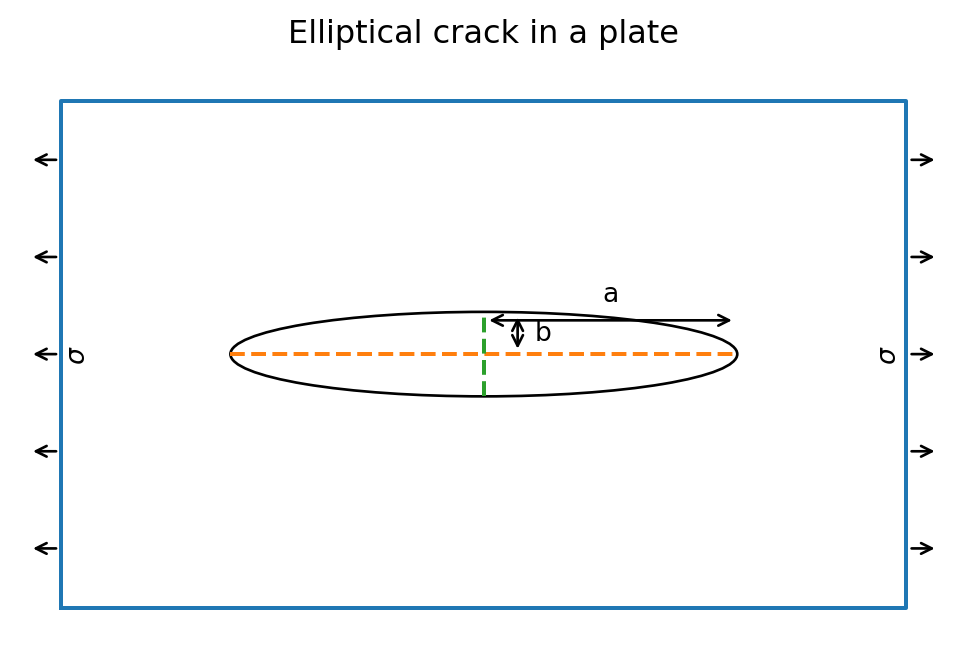
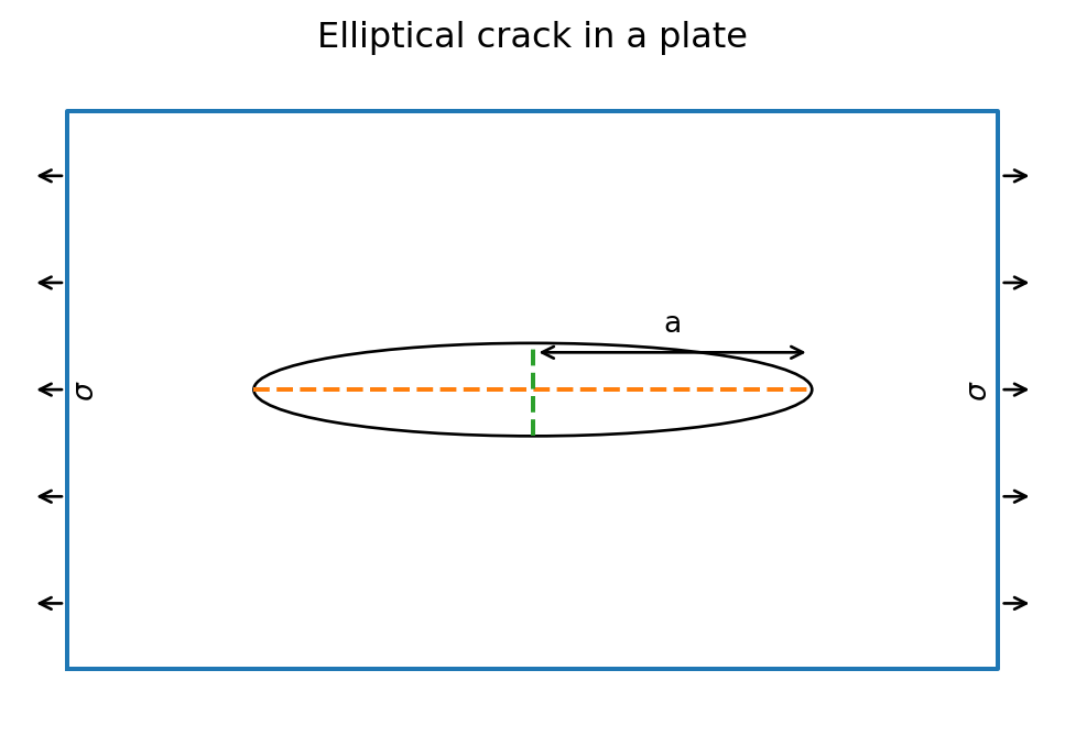
上図のような状態だと、最大引っ張り応力は、Inglis (n.d.) によって示されるように、
\[
\sigma_{max} = \sigma \left( 1 + 2\frac{a}{b} \right)
\]
になる。曲率半径 \(ρ = \frac{b^2}{a}\) を用いると、
\[
\sigma_{max} = \sigma \left( 1 + 2\sqrt{\frac{a}{\rho}} \right) \approx 2\sigma \sqrt{\frac{a}{\rho}}
\]
最後の近似は鋭い亀裂の場合のこと。これから先は鋭い亀裂について考える。
亀裂先端では、与えられた応力よりも増幅された応力 \(\sigma_{max}\) が働くことになる。亀裂が進展するためには、この応力が材料の理想破壊強度 \(\sigma_0\) を超える必要がある。すなわち、
\[
2\sigma \sqrt{\frac{a}{\rho}} = \sqrt{\frac{E\gamma}{r_0}}
\]
理論的にどれだけ鋭いき裂を考えても、原子1個より細かい曲率は作れないので、\(\rho \sim r_0\) と考える。これを代入すると、
\[
\sigma = \sqrt{\frac{E\gamma}{4a}}
\]
これが亀裂先端で破壊が起きるための遠方応力の条件式である。亀裂長さ \(2a\) が大きくなるほど、必要な応力 \(\sigma\) は小さくなることがわかる。
これまでが、ミクロの世界の話。
Airy関数(マクロな世界の話)
講義の板書だけで理解するのは難しかった。なので、調べて考えた結果もざっくばらんにまとめる。
Airy関数は、2次元の弾性体における応力場を記述するための数学的な道具である。2次元の弾性体では、応力テンソルの成分は互いに独立ではなく、互いに関連している。この関係を満たすために、Airy関数 \(\phi(x, y)\) を導入する。
具体的には
\[
\begin{aligned}
\sigma_{xx} &= \frac{\partial^2 \phi}{\partial y^2} \\
\sigma_{yy} &= \frac{\partial^2 \phi}{\partial x^2} \\
\sigma_{xy} &= -\frac{\partial^2 \phi}{\partial x \partial y}
\end{aligned}
\]
こうやって定義しておけば、釣り合いが取れるわけだ。つまり次の式が自動で成立する。
\[
\frac{\partial \sigma_{xx}}{\partial x} + \frac{\partial \sigma_{xy}}{\partial y} = 0
\]
で、 \(\nabla ^2 \phi = \sigma_{xx} + \sigma_{yy}\) という値が、ある点においての応力の和で、物体が滑らかだという条件は、この式で満たされる。
\[\nabla^2 \qty( \nabla ^2 \phi ) = 0\]
で、これを色んな境界条件で解いた解のうち、
コードはこちら
import numpy as np
import matplotlib.pyplot as plt

# Parameters (normalized)
sigma = 1.0
a = 1.0

# Domain (avoid the singularity exactly at x=±a)
x_left  = np.linspace(-3*a, -1.001*a, 1500)
x_right = np.linspace( 1.001*a,  3*a, 1500)
x = np.concatenate([x_left, x_right])

# Crack-front normal stress along x-axis
sigma_y = sigma * np.abs(x) / np.sqrt(x**2 - a**2)

plt.figure()
plt.plot(x, sigma_y, label=r'$\sigma_y(x)=\sigma\,|x|/\sqrt{x^2-a^2}$')
plt.axhline(sigma, linestyle='--', label=r'far-field $\sigma$')
plt.axvline(-a, linestyle='--')
plt.axvline(a, linestyle='--')

# Schematic: crack on the x-axis (drawn below the plot)
y_schem = -0.25
plt.plot([-a, a], [y_schem, y_schem], linewidth=6, solid_capstyle='butt', label='crack (length 2a)')

# Annotations
plt.text(a, y_schem+0.04, r'$a$', ha='center', va='bottom')
plt.text(2.85*a, sigma*1.02, r'$\sigma$', ha='right', va='bottom')

plt.ylim(y_schem-0.2, 8)   # show divergence trend without going infinite
plt.xlim(0, 3*a)
plt.xlabel('x (normalized)')
plt.ylabel(r'$\sigma_y/\sigma$')
plt.title('Crack-front stress distribution + schematic (normalized)')
plt.grid(True)
plt.legend()
plt.show()
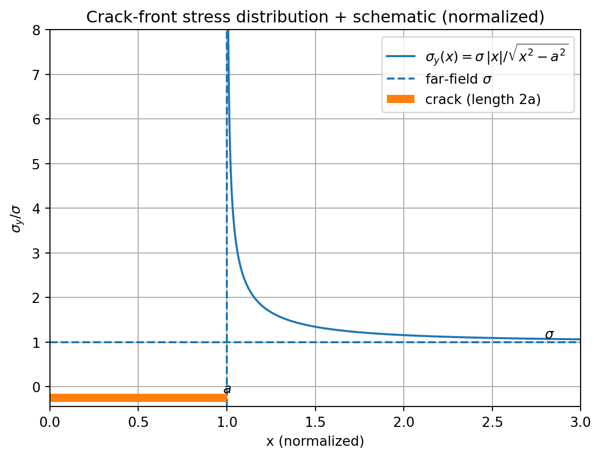
境界で応力が無限に集中して、遠方では一定の応力 \(\sigma\) に収束するようなものがある。これが亀裂先端の応力場のモデルになる。
え、前の節じゃ鋭い亀裂の応力集中は \(\sigma_{max} = 2\sigma \sqrt{\frac{a}{\rho}}\) じゃなかったのかって? そうなんだけど、あれはミクロの話で、こっちはマクロの話だから、無限大っていうモデルを採用してるってさ。
\[
\sigma_y(x) = \sigma \frac{|x|}{\sqrt{x^2 - a^2}}
\]
亀裂近傍における \(x \approx a\) のとき、応力は次の式になる。
\[
\sigma_y(x) \approx \sigma \frac{a + \Delta}{(a + \Delta)^2 - a^2}^{1/2} = \sigma \frac{a + \Delta}{(2a\Delta + \Delta^2)^{1/2}} \approx \sigma \sqrt{\frac{a}{2 \Delta}}
\]
つまりは、 \(\Delta\) が小さければ応力はどんどん集中するわけだけど、実際には無限の応力は存在しない。これはあくまでも、「亀裂先端近傍の応力は非常に大きくなる」という事実を示していて、どのタイミングで破壊が起きるかは \(\sigma\) をデカくして行くことによって決まってくる。
ここで、応力拡大係数を次の式で定義する。変数は \(x \to \Delta\) に変えて書く。
\[
K_{\mathrm{I}} = \lim_{\Delta \to 0} \qty[ \sigma_y(\Delta) \sqrt{2 \pi \Delta} ] = \sigma \sqrt{\pi a}
\]
と定義する。この定義の理由は、 \(\sqrt{\text{応力}} \times \sqrt{\text{長さ}}\) で初めて \(\Delta\) によらない数になるから。
\(\sigma_{\mathrm{max}}\) で扱うと、穴の形や原子構造とか諸々のファクター全てを含む形で決まってくるから、材料的な定数として扱えない。
ところが、 \(K_{\mathrm{I}}\) は亀裂長さ \(a\) と遠方応力 \(\sigma\) のみで決まるので、材料的な定数として扱いやすい。
\(\pi\) は一周で積分することによってできるらしいが、こっちの方はよくわからん。
そうすることによって、破壊される際の \(K_{\mathrm{I}}\) の値を \(K_{\mathrm{IC}}\) として材料定数として扱うことができる。
\[
K_{\mathrm{IC}} = \sigma_{\mathrm{破壊時}} \sqrt{\pi a}
\tag{1}\]
となる。この \(K_{\mathrm{IC}}\) を破壊靭性と呼ぶ。
| \(K_{\mathrm{I}}\) |
\(\mathrm{MPa}\cdot\mathrm{m}^{1/2}\) |
応力拡大係数 |
| \(K_{\mathrm{IC}}\) |
\(\mathrm{MPa}\cdot\mathrm{m}^{1/2}\) |
破壊靭性 |
Griffithのエネルギー論
ここまでは、亀裂周辺で応力がどのように働くかのモデル化で破壊の条件を考えたわけだが、次はエネルギー論的に破壊の条件を考える。
コードはこちら
import matplotlib.pyplot as plt
from matplotlib.patches import Ellipse
import numpy as np

# 板のサイズ(適当なスケール)
width, height = 10, 6

fig, ax = plt.subplots(figsize=(8, 4))

# 板(長方形)の外枠
ax.plot([0, width, width, 0, 0], [0, 0, height, height, 0])

# 楕円き裂の中心
center_x, center_y = width / 2, height / 2

# 楕円き裂の半長軸 a と半短軸 b
a = 3.0   # x方向(き裂長さの半分)
b = 0.5   # y方向

# 楕円き裂
ellipse = Ellipse((center_x, center_y), 2*a, 2*b, fill=False)
ax.add_patch(ellipse)

# 主軸(a方向)・副軸(b方向)を点線で表示
ax.plot([center_x - a, center_x + a], [center_y, center_y], linestyle='--')
ax.plot([center_x, center_x], [center_y - b, center_y + b], linestyle='--')

# a のラベル
ax.annotate(
    "", xy=(center_x + a, center_y + 0.4), xytext=(center_x, center_y + 0.4),
    arrowprops=dict(arrowstyle="<->")
)
ax.text(center_x + a/2, center_y + 0.55, "a", ha="center", va="bottom")

# 遠方引張応力 σ を左・右に描く
y_pos = np.linspace(0.7, height - 0.7, 5)
for y in y_pos:
    # 左側の矢印(→)
    ax.annotate("", xy=(-0.4, y), xytext=(0, y),
                arrowprops=dict(arrowstyle="->"))
    # 右側の矢印(←)
    ax.annotate("", xy=(width + 0.4, y), xytext=(width, y),
                arrowprops=dict(arrowstyle="->"))

ax.text(0.2, height/2, r"$\sigma$", ha="center", va="center", rotation=90)
ax.text(width - 0.2, height/2, r"$\sigma$", ha="center", va="center", rotation=90)

# 体裁整え
ax.set_aspect("equal")
ax.set_xlim(-0.5, width + 0.5)
ax.set_ylim(-0.5, height + 0.5)
ax.axis("off")
ax.set_title("Elliptical crack in a plate")

plt.show()
これで、まずは亀裂が進行することによって増えるエネルギーは、
\[
W_\mathrm{e} = \frac{\pi a^2 \sigma^2}{E}
\]
となる。次元的にエネルギーの単位になる。実際の計算は無理だった。
次に表面が増えるのでその分の表面エネルギーは次の式になる。
\[
W_\mathrm{s} = 4 a \gamma
\]
コードはこちら
import numpy as np
import matplotlib.pyplot as plt

# --- Parameters (dimensionless / schematic) ---
E = 1.0
gamma = 0.18
sigma = 0.45

# Crack half-length a
a = np.linspace(0, 1.2, 600)

# Griffith model (schematic, plane stress-like)
We = (np.pi * a**2 * sigma**2) / E          # elastic energy released (positive quantity)
Ws = 4 * a * gamma                          # surface energy cost
U = -We + Ws                                # total potential energy change

# Critical crack length from dU/da = 0  -> 4γ - 2πσ^2 a / E = 0
ac = (2 * E * gamma) / (np.pi * sigma**2)

# --- Plot 1: Energy balance diagram ---
plt.figure()
plt.plot(a, -We, label=r"$-W_e$  (elastic energy release)")
plt.plot(a, Ws,  label=r"$W_s$   (surface energy cost)")
plt.plot(a, U,   label=r"$U(a)=-W_e+W_s$")
plt.axvline(ac, linestyle="--")
plt.text(ac, np.interp(ac, a, U), r"  $a_c$", va="bottom")

plt.xlabel(r"crack half-length $a$")
plt.ylabel("energy (schematic units)")
plt.title("Griffith energy balance (schematic)")
plt.grid(True)
plt.legend()
plt.ylim(min(U.min(), (-We).min()) * 1.1, max(Ws.max(), U.max()) * 1.1)
plt.xlim(0, a.max())
plt.show()
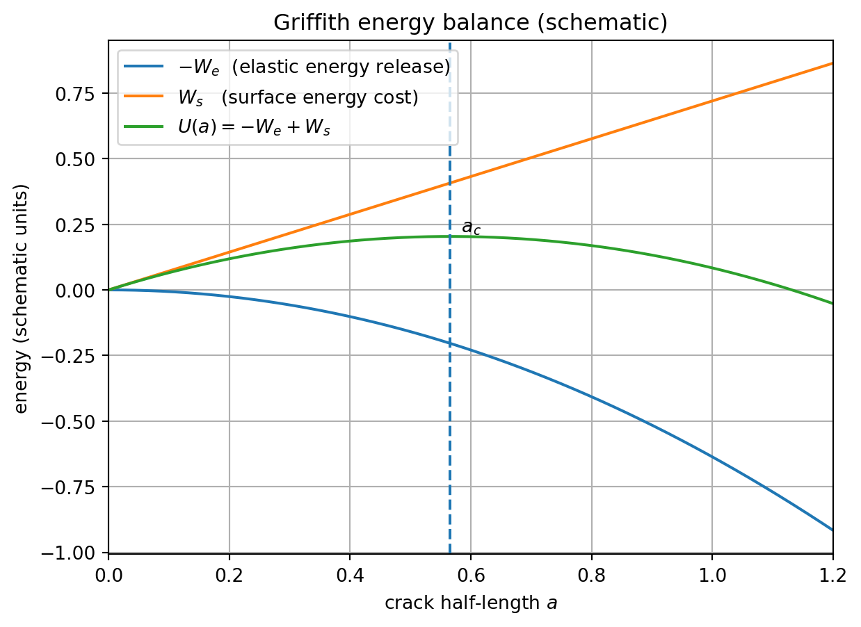
\[
U = -W_\mathrm{e} + W_\mathrm{s} = -\frac{\pi a^2 \sigma^2}{E} + 4 a \gamma
\]
このグラフを見ればわかるのが、極大点の \(a_\mathrm{c}\) を超えると、同じ応力があれば亀裂が勝手に伸びていくことになる。
逆に、その前だと、亀裂は力を加え続けなければ進まない。
\[
\begin{aligned}
\dv{U}{a}(a_\mathrm{c}) &= -\frac{2\pi a \sigma^2}{E} + 4 \gamma = 0 \\
a_\mathrm{c} &= \frac{2 E \gamma}{\pi \sigma^2}
\end{aligned}
\]
また、見方を変えれば、ある亀裂長さ \(a\) に対して、亀裂が進展するための応力は、
\[
\sigma_\mathrm{c} = \sqrt{\frac{2 E \gamma}{\pi a}}
\tag{2}\]
となる。これは、Inglisの応力集中を考えたときの式と係数以外は一致する。当然だ。だって、Inglisの応力集中もエネルギー論も、同じ物理現象を説明しているし、また、かなり大雑把なモデル化をしているから、多少の違いは出てくる。
\(2\gamma = \Gamma\) と表面エネルギーを置き換えると、
\[
\sigma_\mathrm{c} = \sqrt{\frac{E \Gamma}{\pi a}}
\]
この \(\Gamma\) というのは、エネルギー解放率と呼ばれているのだが、その理由は、この亀裂の進展を片方だけで見た時、
\[
U = -\frac{\pi a^2 \sigma^2}{2E} + a \Gamma
\]
と、半分の値になってて、そのうちの弾性エネルギーがどれだけ解放されるかを示しているから。
Equation 1 で示される \(K_{\mathrm{IC}}\) を用いると、破壊の条件式は次のように書ける。
\[
\begin{aligned}
K_{\mathrm{IC}} &= \sqrt{E \Gamma} \\
\Gamma &= \frac{K_{\mathrm{IC}}^2}{E}
\end{aligned}
\]
雑まとめ
| 磁粉探傷試験 |
MT |
磁化による漏洩磁束に磁粉を付着させて欠陥を可視化 |
表面・表面直下のき裂 |
深部内部欠陥、非磁性材料 |
✕ |
| 浸透探傷試験 |
PT |
毛細管現象により表面開口欠陥に浸透液を浸透させ検出 |
表面開口き裂 |
内部欠陥、表面非開口欠陥 |
✕ |
| 放射線透過試験 |
RT |
X線・γ線の透過量差を画像として検出 |
体積欠陥(ブローホール、スラグ巻込み) |
面状き裂、欠陥面が薄い場合 |
△ |
| 超音波探傷試験 |
UT |
超音波の反射・散乱を利用して内部欠陥を検出 |
内部き裂、面状欠陥(割れ、未溶着) |
表面極近傍欠陥、粗大組織 |
◎ |
問題
応力拡大係数と破壊靱性
ひっぱり強度 \(\sigma = 800 \mathrm{MPa}\) で破壊靱性 \(K_{\mathrm{IC}} = 50 \mathrm{MPa}\cdot\mathrm{m}^{1/2}\) の材料に、長さ \(2a = 10 \mathrm{mm}\) の亀裂があるとする。 この材料に \(400 \mathrm{MPa}\) の応力がかかったとき、亀裂は進展するか? 形状係数は \(Y=1\) とする。
Equation 1 から、破壊の条件は
\[
\begin{aligned}
\sigma_{\mathrm{破壊時}} &= \frac{K_{\mathrm{IC}}}{Y \sqrt{\pi a}} \\
&= \frac{60 \mathrm{MPa}\cdot\mathrm{m}^{1/2}}{1 \cdot \sqrt{\pi \cdot 5 \times 10^{-3} \mathrm{m}}} \\
&\approx 478.64 \mathrm{MPa}
\end{aligned}
\]
応力 \(400 \mathrm{MPa}\) はこれを下回るので、亀裂は進展しない。
Griffithのエネルギー論による亀裂進展条件
ある脆性材料の表面エネルギーが \(\gamma = 1.0 \mathrm{J/m^2}\)、ヤング率が \(E = 70 \mathrm{GPa}\) であるとする。この材料に存在する長さ \(2a = 2.0 \mu \mathrm{m}\) の亀裂が進展するために必要な最小の引張応力を求めよ。ただしGriffithのエネルギー論を用いるものとする。
Equation 2 から、
\[
\begin{aligned}
\sigma_\mathrm{c} &= \sqrt{\frac{2 E \gamma}{\pi a}} \\
&= \sqrt{\frac{2 \times 70 \times 10^9 \mathrm{Pa} \times 1.0 \mathrm{J/m^2}}{\pi \times 1.0 \times 10^{-6} \mathrm{m}}} \\
&\approx 2.11 \times 10^6 \mathrm{Pa} = 211 \mathrm{MPa}
\end{aligned}
\]
Paris則
幅 \(W\) 、厚さ \(t\) の平板に、繰り返しひっぱり荷重 \(P\) がかかる。次に定数の一覧が与えられている。
| \(P_{\mathrm{max}} = 50\) |
\(\mathrm{kN}\) |
最大荷重 |
| \(P_{\mathrm{min}} = 0\) |
\(\mathrm{kN}\) |
最小荷重 |
| \(A = 500\) |
\(\mathrm{mm}^2\) |
平板面積 |
| \(a = 1.0\) |
\(\mathrm{mm}\) |
亀裂長さの半分 |
| \(C = 10^{-11},\ m=4\) |
なし |
材料定数 |
| \(a_{\mathrm{f}} = 20\) |
\(\mathrm{mm}\) |
限界亀裂長さ |
この時、疲労破壊に要する繰り返し荷重回数 \(N_{\mathrm{f}}\) を求めよ。
Parisの法則によれば、疲労亀裂の進展速度 \(da/dN\) は応力拡大係数範囲 \(\Delta K\) の関数として次のように表される。
\[
\dv{a}{N} = C (\Delta K)^m
\]
\[
\begin{aligned}
\frac{\dd a}{C (\Delta \sigma \sqrt{\pi a})^m} &= \dd N \\
\int_{a_0}^{a_f} \frac{\dd a}{C (\Delta \sigma \sqrt{\pi a})^m} &= \int_0^{N_f} \dd N \\
N_f &= \frac{1}{C (\Delta \sigma \sqrt{\pi})^m} \int_{a_0}^{a_f} a^{-m/2} \dd a \\
&= \frac{1}{C (\Delta \sigma \sqrt{\pi})^m} \cdot \frac{2}{2 - m} \left( a_f^{1 - m/2} - a_0^{1 - m/2} \right) \\
&= \frac{1}{10^{-11} (500 \times 10^3 / 500 \times \sqrt{\pi})^4} \cdot \frac{2}{2 - 4} \left( (20 \times 10^{-3})^{1 - 4/2} - (1.0 \times 10^{-3})^{1 - 4/2} \right) \\
&\approx 1.16 \times 10^5
\end{aligned}
\]
コードはこちら
import numpy as np

# --- Parameters ---
P_max = 50e3        # 最大荷重 (N)
P_min = 0            # 最小荷重 (N)
A = 500e-6           # 平板面積 (m^2)
a0 = 1.0e-3          # 亀裂長さの半分 (m)
af = 20e-3           # 限界亀裂長さ (m)
C = 1e-11            # 材料定数
m = 4                 # 材料定数

# --- Calculations ---
delta_sigma = (P_max - P_min) / A  # 応力範囲 (Pa)
N_f = (1 / (C * (delta_sigma * np.sqrt(np.pi))**m)) * (2 / (2 - m)) * (af**(1 - m/2) - a0**(1 - m/2))
print(f"疲労破壊に要する繰り返し荷重回数 N_f ≈ {N_f:.2e}")
疲労破壊に要する繰り返し荷重回数 N_f ≈ 9.63e-20
Basquin則, Miner則
ある合金の疲労試験の結果が以下のデータとなった。
\[
\begin{aligned}
N & : 10^5, 10^6 \\
\Delta \sigma /2 & : 400, 300 \quad (\mathrm{MPa})
\end{aligned}
\]
応力振幅が \(250 \mathrm{MPa}\) のときの疲労寿命 \(N\) を求めよ。
次に同じ材料に対して、応力振幅 \(400 \mathrm{MPa}\) で \(5 \times 10^4\) 回与えたのちに、応力振幅 \(300 \mathrm{MPa}\) で疲労負荷を与えたとき、Miner則に基づいて破壊に至るまでの繰り返し回数を求めよ。
Basquin則は次の式の通り。
\[
\qty(\frac{\Delta \sigma}{2})^b N_{\mathrm{f}} = C
\]
Miner則は次の式の通り。
\[
\sum_i \frac{N_i}{N_{\mathrm{f},i}} = 1
\]
\[
\begin{aligned}
200^b \cdot 10^5 &= 150^b \cdot 10^6 \\
b &= \frac{\log_{10} (10)}{\log_{10} (200/150)} \approx 8 \\
C &= 200^{6.58} \cdot 10^5 \approx 4.00 \times 10^{13} \\
N_{\mathrm{f}} &= \frac{C}{(125)^b} \approx 4.3 \times 10^6
\end{aligned}
\]
次に、
\[
\begin{aligned}
\frac{5 \times 10^4}{N_{\mathrm{f},1}} + \frac{N_2}{N_{\mathrm{f},2}} &= 1 \\
\frac{5 \times 10^4}{10^5} + \frac{N_2}{10^6} &= 1 \\
N_2 &\approx 5 \times 10^5
\end{aligned}
\]
ネルンストの式
\(\mathrm{pH} = 0,\ T = 298 \mathrm{K}\) の水溶液中の鉄の腐食を考える。ただし \([\mathrm{Fe}^{2+}] = 10^{-6} \mathrm{mol/L}\) とする。
- 鉄の溶解反応と水素発生反応の平衡電位をネルンストの式を用いて求めよ。ただし鉄の標準電極電位は \(E^\circ (\mathrm{Fe}^{2+}/\mathrm{Fe}) = -0.44 \mathrm{V}\) とする。
- ターフェル式を用いて、腐食電流密度を求めよ。ただし、アノード反応のターフェル定数 \(E = -0.62 + 0.06 \log_{10} i\)、カソード反応のターフェル定数 \(E = -0.30 - 0.10 \log_{10} i\) として、\(i\) の単位は \(\mu \mathrm{A/cm^2}\) とする。
- この材料の一年あたりの減肉深さを算出せよ。
ネルンストの式は次の通り。
\[
\begin{aligned}
\Delta G &= n F E \\
E &= E^\circ - \frac{RT}{nF} \ln Q \\
&= E^\circ - \frac{0.059}{n} \log_{10} Q
\end{aligned}
\]
- 鉄の溶解反応は、 \[
E = -0.44 - \frac{0.0592}{2} \log_{10} \frac{1}{10^{-6}} = -0.617 \mathrm{V}
\] 水素発生反応は、 \(0 \mathrm{V}\) 。以上から、鉄の溶解反応の方が電位が低いので、腐食は鉄の溶解反応が支配的である。
- \[
\begin{aligned}
-0.62 + 0.06 \log_{10} i &= -0.30 - 0.10 \log_{10} i \\
0.16 \log_{10} i &= 0.32 \\
\log_{10} i &= 2 \\
i &= 100 \mu \mathrm{A/cm^2}
\end{aligned}
\]
- \[
\begin{aligned}
\frac{Miy}{zF\rho} = 1.16 \ \mathrm{mm / year}
\end{aligned}
\]
弾性体の運動方程式
次の式を導出し、 \(E=206 \mathrm{GPa}\) 、密度 \(\rho=7.85 \times 10^3 \mathrm{kg/m^3}\) の材料において、波動速度を求めよ。
\[
\frac{\partial^2 u}{\partial t^2} = c^2 \frac{\partial^2 u}{\partial x^2}
\]
また、長さ \(L = 2.0 \mathrm{m}\) の鉄棒の両端にAEセンサーを取り付けた時、棒上の位置 \(x\) で破壊が発生した。計測の結果、AEセンサーには到達時間差 \(\Delta t = 0.2 \mathrm{ms}\) で信号が到達した。このとき、破壊が発生した位置 \(x\) を求めよ。
\[
\begin{aligned}
A\rho \dd x \pdv[2]{u}{t} &= A\pdv{\sigma}{x} \dd x \\
\sigma &= E \pdv{u}{x} \\
\therefore \rho \pdv[2]{u}{t} &= E \pdv[2]{u}{x} \\
c &= \sqrt{\frac{E}{\rho}} = \sqrt{\frac{206 \times 10^9 \mathrm{Pa}}{7.85 \times 10^3 \mathrm{kg/m^3}}} \\
&\approx 5.12 \times 10^3 \mathrm{m/s} \\
\Delta t &= \frac{x}{c} - \frac{L - x}{c} \\
x &= \frac{c \Delta t + L}{2} \approx 0.49 \mathrm{m}
\end{aligned}
\]
Back to top